Introduction
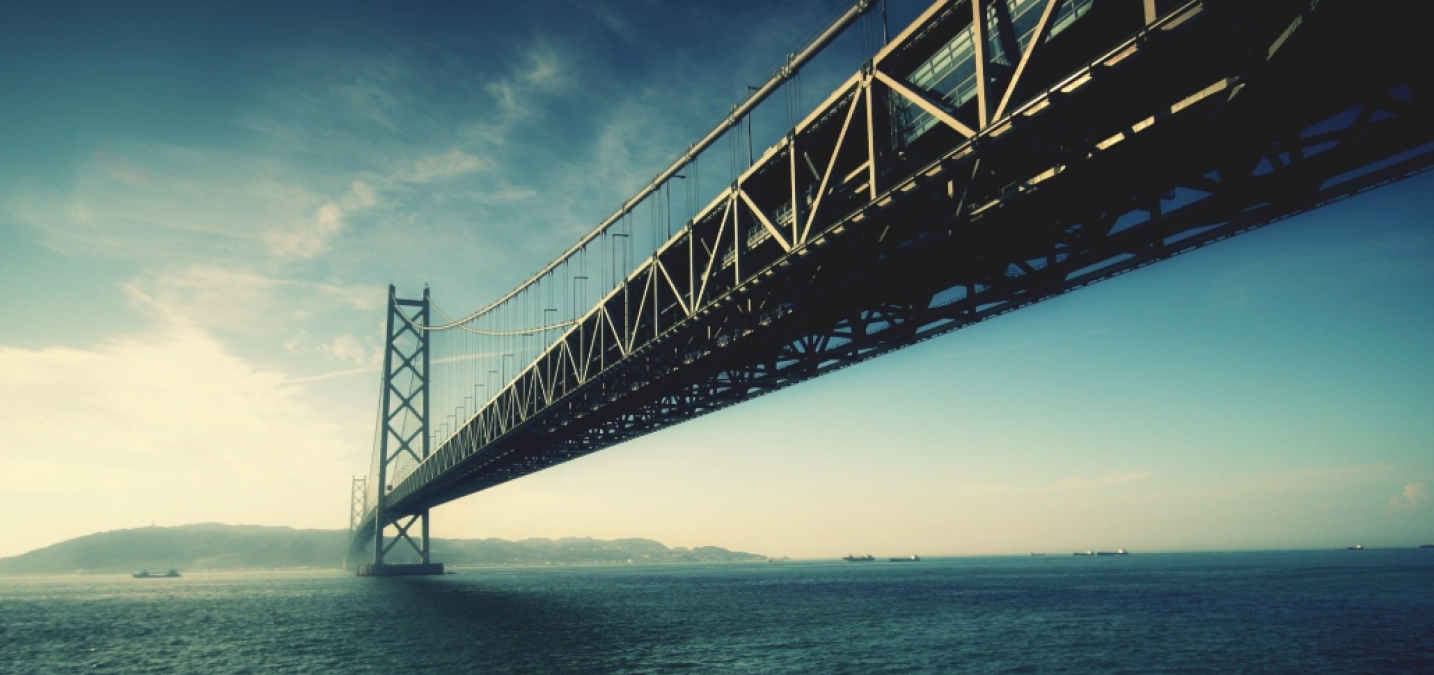
The Akashi Kaikyō is a suspension bridge, which links the city of Kobe on the Japanese mainland of Honshu to Iwaya on Awaji Island. It was completed in 1998 and has the longest central span of any suspension bridge in the world. The entire bridge has three spans. The central span is 1,991 m and the two other sections are each 960 m. Overall the bridge measures 3,911 m in length. The two towers were originally 1,990 m apart, but the Great Hanshin earthquake on January 17, 1995, moved the towers so much (only the towers had been erected at the time) that the span had to be increased by 1 m.
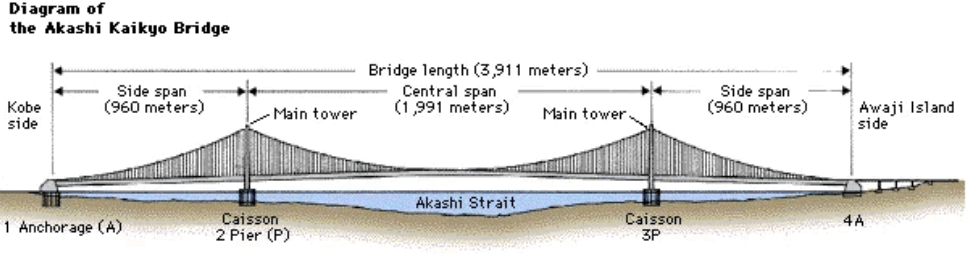
In Figure 1, the dimensions of the Akashi Kaikyō bridge can be seen. To build the FEM model, a more detailed geometry of the bridge was needed. We found some of the publicly available data on the Akashi Kaikyō bridge structure. The sketches can be seen in Figure 2.

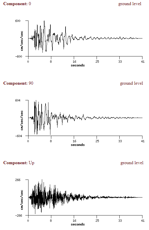
The main goal of this case study was to calculate the response of the bridge during the Great Hanshin earthquake. We managed to find the data from the seismograph, which are presented in Figure 3.
Geometry and Mesh
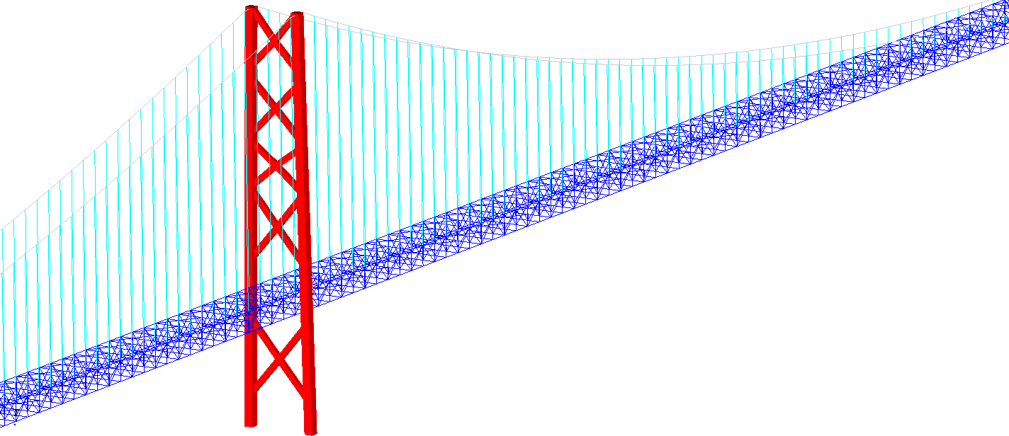
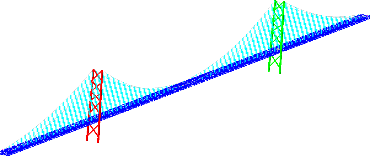
Because of the complexity of the structure, we decided to prepare two separate numerical models. The global model consisted of the entire bridge structure. Main towers, cables and the main beam structure with the roadway. The majority of the structure was modeled with beam elements. The wires, the main cables, and the main bean structure were all modeled with 1D beam elements. Upon completion, the global finite element model consisted of nearly 500.000 elements and can be seen in Figure 4.
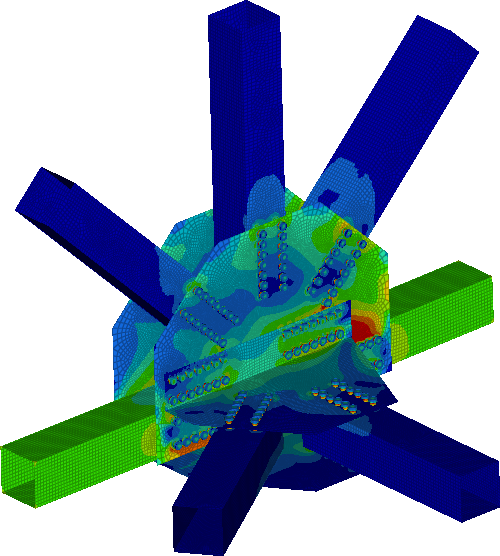
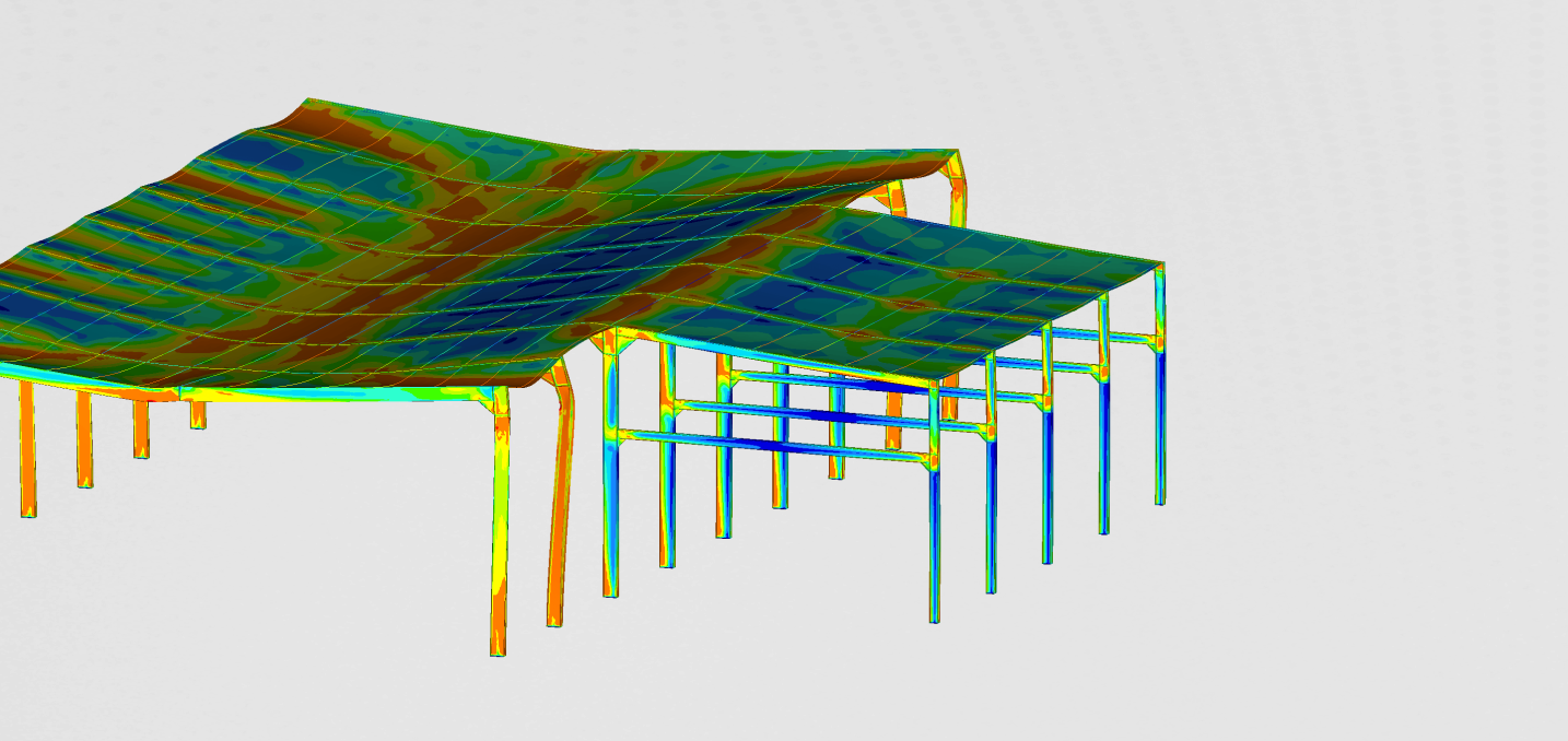
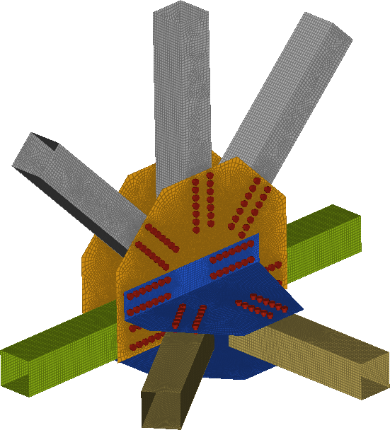
The second, more detailed finite element model, was built to evaluate the structural integrity of the most stressed areas of the bridge. This turned out to be the joint where vertical and horizontal beams of the structure meet. The detailed model was built with a solid and shell finite element. It contained detailed beam geometry, together with all the bolts and plates. The loads and BC for this detailed model were taken from the global model. They came in the form of forces and moments in each beam. The detailed model of the bridge can be seen in Figure 5:
Loads and Boundary Conditions
Simulation methodology, together with loads and boundary conditions is presented below.
Global model
- Static analysis with the gravitational load
- Natural frequency extraction
- Transient dynamics with the base acceleration
Detailed model
- Bolt Preload
- Static analysis with the loads from the global model
For the initial static analysis of the global model, all the cables needed to be pre-tensioned. After the static analysis, the natural frequencies were calculated followed by the transient dynamic analysis. The loading on the global model came in the form of base acceleration. In the detailed model, the bolt pretension was executed first, followed by the static analysis.
Results
Natural frequencies
To determine the upper limit of the natural frequency extraction, the FFT of the base acceleration signal was performed. The FFT shows that the excitation spectrum of the bridge is mostly present up to 10 Hz. This was also the upper limit for natural frequency extraction.
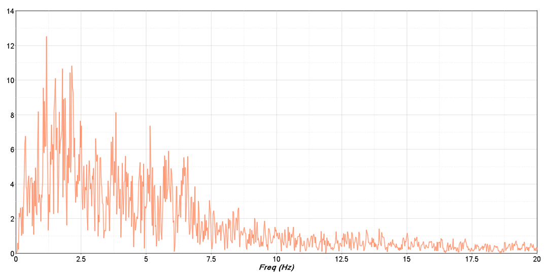
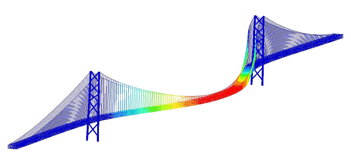
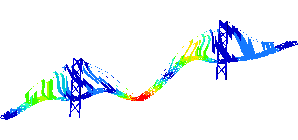
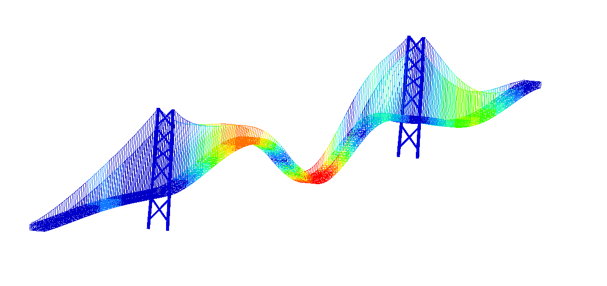
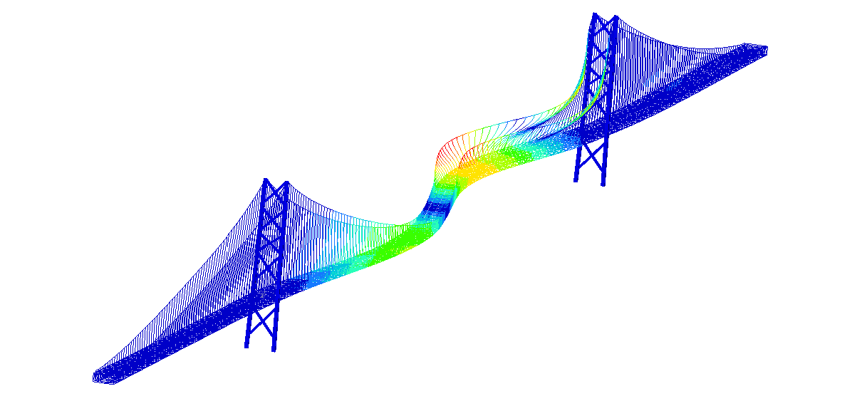
Figure 7: Four most important natural frequencies
Transient dynamics
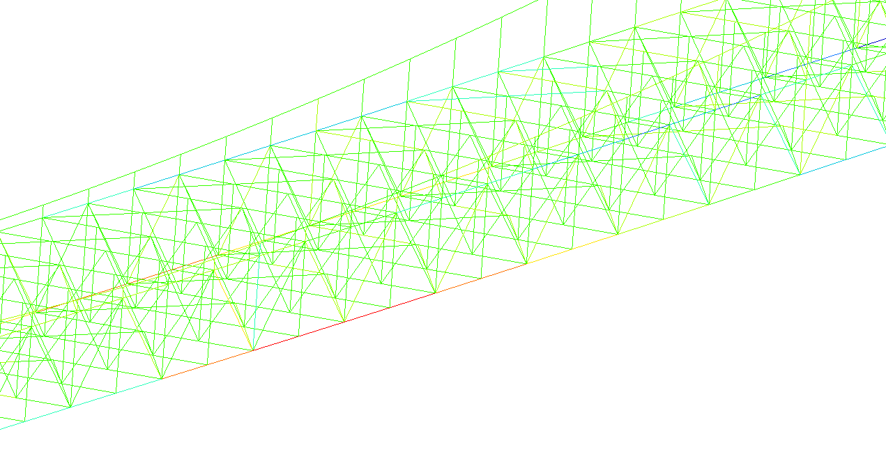
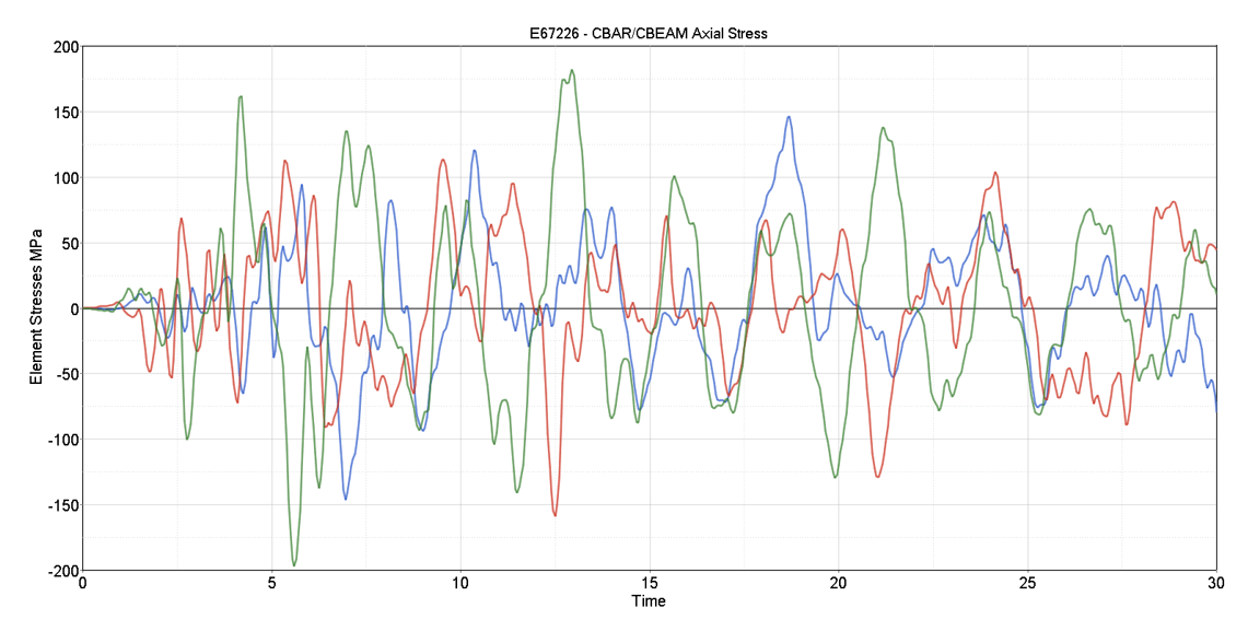
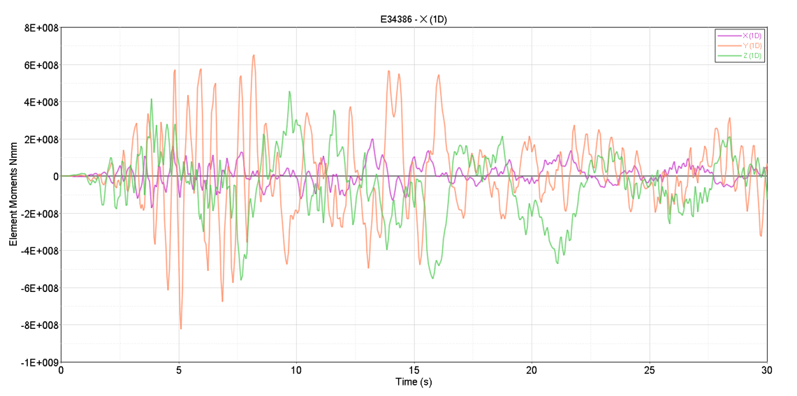
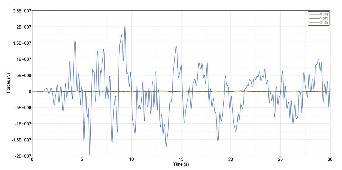
In the video below the transient response of the bridge can be observed. In Figure 8 the most stressed area of the bridge is identified. This area was later considered in the detailed model. Forces and moments acting on the beam are presented in the graphs below.
On Figure 8 the most stressed area of the bridge is identified. This link was also the one considered in the later detailed model. Further more the beam forces and momentums were presented on the graphs below.
Static analysis
Detailed stresses on the joint, during static analysis, can be seen in the Figure12. Longitudinal beams turned out to be the most stressed part of the main structure.